30 Day Chart Challenge- Flora and Fauna

How Large are Different Types of Turtles?

It is Day 3 of the #30DayChartChallenge. More info can be found at the challenge’s Github page. Today’s theme is flora and fauna. I found a trove of fascinating data at Global Assessment of Reptile Distributions. I chose the dataset on body size/ mass from the paper: “Different solutions lead to similar life history traits across the great divides of the amniote tree of life.” by Shai Meiri, Gopal Murali, Anna Zimin, Lior Shak, Yuval Itescu, Gabriel Caetano, and Uri Roll (Journal of Biological Research-Thessaloniki), 202128: 3.

Okay, let’s go. I’m going to keep the libraries to a minimum. That’s always my goal, but yet I ended up with 6!

library(tidyverse)
library(skimr)
library(gt)
library(ggthemes)
library(cowplot)
library(magick)

fauna <- read_csv("animals.csv", show_col_types = FALSE)

I’m going to change the class, clade, order, family and bionomial_2020 to factors. I’m keeping those columns and the mass and discarding the rest.

fauna_cleaned <- fauna %>%
  select(Class:`body mass (g)`) %>%
  select(-`binomial_(original files)`) %>%
  rename(mass_g = `body mass (g)`, name = binomial_2020) %>%
  mutate(Class = factor(Class),
         Clade = factor(Clade),
         order = factor(order),
         family = factor(family),
         name = factor(name))

So, let’s see what kind of data we have.

table1 <- fauna_cleaned %>%
  count(Class)

gt(table1)

Class	n
Aves	9534
Mammalia	5840
Reptilia	11240

We have data on more than just reptiles, the dataset includes information about birds and mammals as well. But I’m only interested in reptiles.

reptiles <- fauna_cleaned %>%
  filter(Class == "Reptilia")

table2 <- reptiles %>%
  count(Clade, order)

gt(table2)

Clade	order	n
Crocodylia	Crocodylia	24
Rhynchocephalia	Rhynchocephalia	1
Squamata	Squamata (Amphisbaenia)	195
Squamata	Squamata (Sauria)	6868
Squamata	Squamata (Serpentes)	3837
Testudines	Testudines	315

Everyone knows that turtles are the best type of reptile, so let’s filter even further.

turtles <- reptiles %>% 
  filter(Clade == "Testudines")

table3 <- turtles %>%
  count(order, family)

gt(table3)

order	family	n
Testudines	Carettochelyidae	1
Testudines	Chelidae	53
Testudines	Cheloniidae	6
Testudines	Chelydridae	3
Testudines	Dermatemydidae	1
Testudines	Dermochelyidae	1
Testudines	Emydidae	47
Testudines	Geoemydidae	69
Testudines	Kinosternidae	24
Testudines	Pelomedusidae	18
Testudines	Podocnemididae	8
Testudines	Testudinidae	54
Testudines	Trionychidae	30

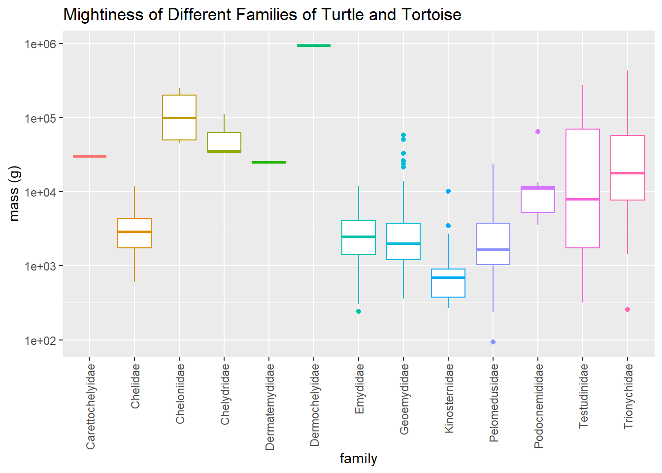
Let’s take a look at how big (or mighty, as some might say) the different families of turtles are. There is a very large range of masses so I’m using a log scale.

ggplot(turtles, aes(x = family, y = mass_g, color = family)) +
  scale_y_log10() +
  geom_boxplot() +
  ggtitle("Mightiness of Different Families of Turtle and Tortoise") +
  ylab("mass (g)") +
  theme(legend.position = "none" , 
        axis.text.x = element_text(angle = 90, vjust = 0.5, hjust = 1))

The heaviest turtles are the giantic leatherback turtles, a species of SEA TURTLE that weigh hundred of kg (around 1,000 lbs). The smallest turtle is the African dwarf mud turtle (Pelusios nanus), family Pelomedusidae, which full grown weighs under 100 grams.

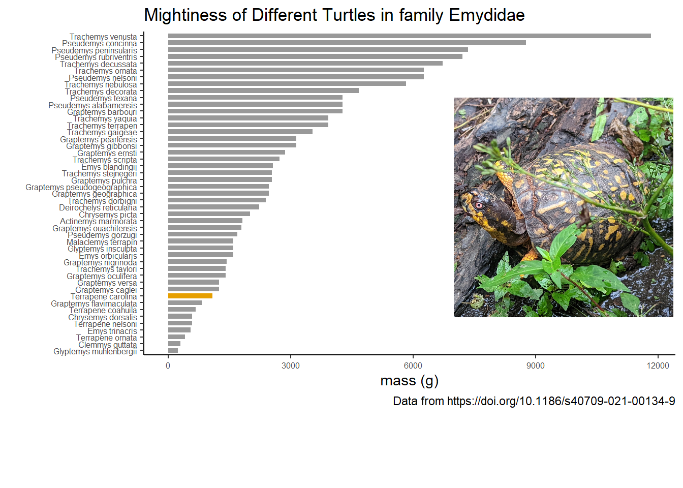
Now let’s look at everyone’s favorite family of turtles, Emydidae. This family is often known as pond or marsh turtles. Filter them out, and add a category for Eastern Box Turtles. I called the variable box_turtle, but I’m only marking Eastern. There are other types of box turtles though not all of them are in Emydidae. Asian box turtle species were reassigned to the family Geoemydidae.

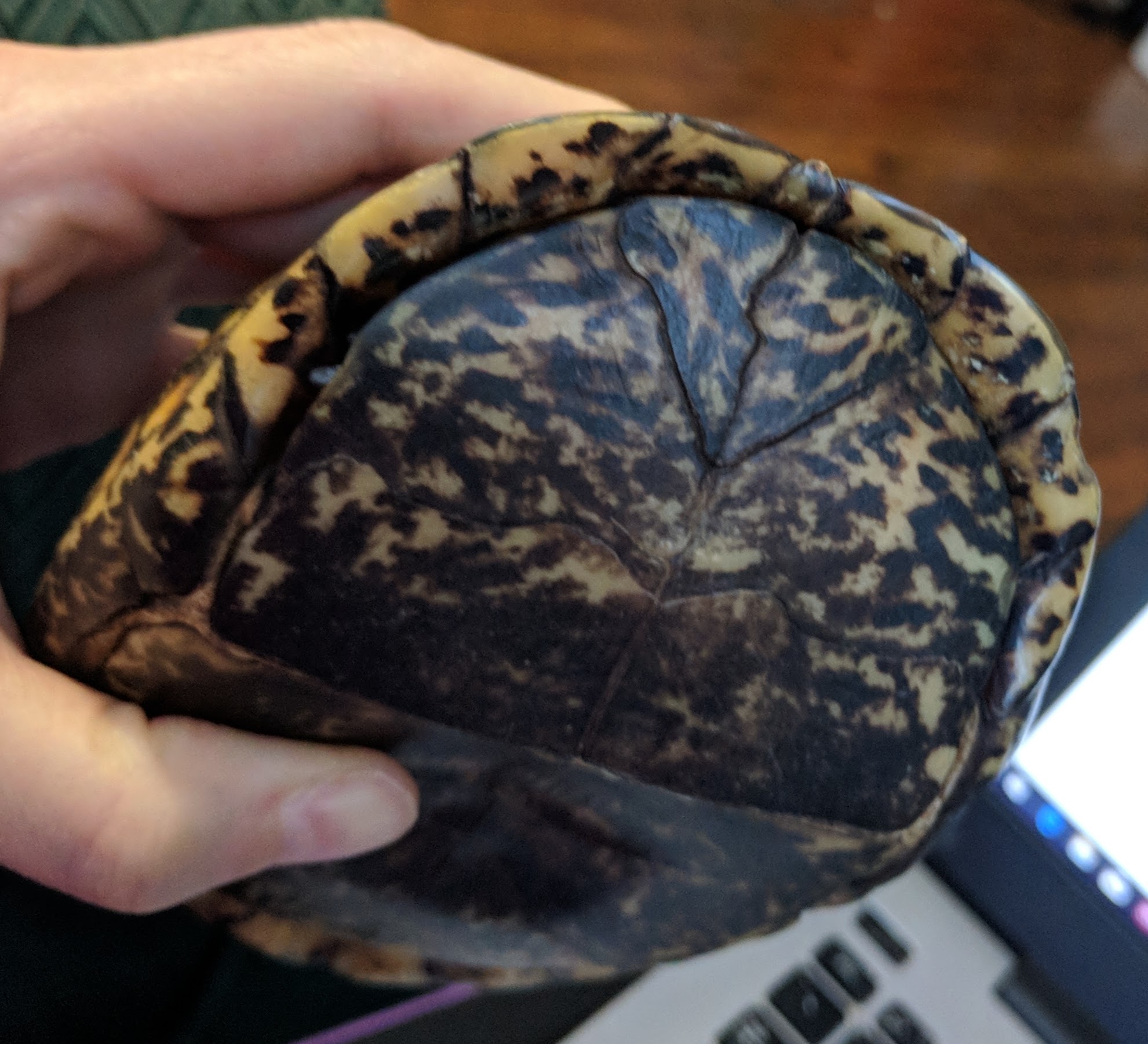
The common name box turtle, arises from the fact that these species have a hinge on the bottom shell, and can close up/ box up completely. Other turtles and tortoises can only pull their bits within their shell.

A closed Eastern Box Turtle

pond_turtles <- turtles %>%
  filter(family == 'Emydidae') %>%
  mutate(box_turtle = ifelse(name == "Terrapene carolina", TRUE, FALSE)) 

Okay, let’s look at mightiness of the turtles in this family.

turtle_plot <- pond_turtles %>%
  ggplot(aes(x = fct_reorder(name, mass_g), y = mass_g, fill = box_turtle)) +
  scale_fill_manual(values=c("#999999", "#E69F00")) +
  geom_col(width = 0.7, position = position_dodge(10)) +
  coord_flip() +
  ylab("mass (g)") +
  xlab("") +
  ggtitle("Mightiness of Different Turtles in family Emydidae") +
  labs(caption = "Data from https://doi.org/10.1186/s40709-021-00134-9") +
  theme_classic() +
  theme(axis.text = element_text(size = 6)) +
  theme(legend.position = "none")


#found how to add an image to my graph on stack overflow
#https://stackoverflow.com/questions/63442933/how-can-i-add-a-logo-to-a-ggplot-visualisation

img <- image_read("pqtk5r.jpg")

# Set the canvas where you are going to draw the plot and the image
ggdraw() +
# Draw the plot in the canvas setting the x and y positions, which go from 0,0
# (lower left corner) to 1,1 (upper right corner) and set the width and height of
# the plot. It's advisable that x + width = 1 and y + height = 1, to avoid clipping # the plot
draw_plot(turtle_plot,x = 0, y = 0.15, width = 1, height = 0.85) +
# Draw image in the canvas using the same concept as for the plot. Might need to 
# play with the x, y, width and height values to obtain the desired result
draw_image(img, x = 0.6, y = 0.35, width = 0.45, height = 0.45) 

Citation

BibTeX citation:

@online{sinks2023,
  author = {Sinks, Louise E.},
  title = {30 {Day} {Chart} {Challenge-} {Flora} and {Fauna}},
  date = {2023-04-03},
  url = {https://lsinks.github.io/posts/2023-04-03-chart-challenge-3/day3.html},
  langid = {en}
}

For attribution, please cite this work as:

Sinks, Louise E. 2023. “30 Day Chart Challenge- Flora and Fauna.” April 3, 2023. https://lsinks.github.io/posts/2023-04-03-chart-challenge-3/day3.html.