#|label: helper-functions
Construct_Freq_Table <- function(word_list) {

#scoring code uses the counting code from

#https://www.r-bloggers.com/2018/12/rrrrs-in-r-letter-frequency-in-r-package-names/
# making the frequency table ----

letters <- unlist(strsplit(word_list[,1], split = ""))
char_frequencies <- as.data.frame(table(letters))

#normalized
common <- max(char_frequencies[,2])
y = (char_frequencies[,2]/common)
char_frequencies$normalized <- y
return(char_frequencies)
}

Scoring_Word <- function(word, freqs = char_frequencies,
                         verbose = FALSE, debug_detail = FALSE){
  letter_vec <-  unlist(strsplit(word, split = ""))
    if (verbose == TRUE)
    {message("I'm in Scoring_words message and scoring: ", word)}

  value <- 0
  for (i in 1:length(letter_vec)) {
    position <- letter_vec[i]== freqs$letters
    value[i] <- freqs$normalized[position]
    if (debug_detail == TRUE)
    {
      print("I am in the scoring loop calculating value: ")
      print(i)
      print(sum(value))

    }

    if (i == length(letter_vec)) {

      return(total <- sum(value))
    }

  }
  }


Scoring_Word_Unique <- function(word, freqs = char_frequencies,
                                verbose = FALSE, debug_detail = FALSE){
  # This does only score on unique letters
  letter_vec <-  unlist(strsplit(word, split = ""))
  unique_letter_vec <- unique(letter_vec)
  #unique_letter_vec <- letter_vec
  if (verbose == TRUE)
  {message("I'm in Scoring_words_Unique and scoring: ", word)}

  value <- 0
  if (length(unique_letter_vec) == 0) {
    return(value)
  } else{
    for (i in 1:length(unique_letter_vec)) {
           position <- unique_letter_vec[i] == freqs$letters
          value[i] <- freqs$normalized[position]
      if (debug_detail == TRUE)
      {
        print("I am in the unique scoring loop calculating value: ")
        print(i)
        print(sum(value))
      }

      if (i == length(unique_letter_vec)) {

        return(total <- sum(value))
      }

    }
  }
}

Removing_Letters <- function(word, chosen_word,
                              verbose = FALSE, debug_detail = FALSE) {
  lvec <- gsub(paste0("[", chosen_word, "]"), "", word)
return(lvec)}Self-Guided Learning through a Wordle Guess Generator: Part 2
This is the current version of the word game guesser. I discussed how I used this project to hone my coding skills in the companion blog post to this one.
I’m not going to walk through this in much detail, but I’m going to point out some of the major lessons I learned as I revised the code. Again, both the initial version and this version are on GitHub in all their messiness.
I learned how to put functions in a separate file and call them from my many script. This can make long code much easier to read. Here, I’ve included the helper functions in-line and commented out the source("code/helper-functions.R") in the main code. I’ve also set up switchable troubleshooting help with verbose and debug_detail parameters in my functions. Setting them to TRUE provide more info as the functions are executed.
I finally did figure out how to make variables the types I wanted. I also replaced several loops with map functions from purrr. I also made a reshaped version of my dataframe using pivot_longer from tidyr. Reshaping data is a really useful skill, but might be a bit confusing at first. So I certainly wanted to make sure I could do it correctly. The reshaped data is used to make a nice density plot later.
# Loading libraries and data ----
library("tidyverse")


#from https://www-cs-faculty.stanford.edu/~knuth/sgb-words.txt
word_list <-
  read.table("C:/Users/drsin/OneDrive/Documents/R Projects/Word-Games/input/sgb-words.txt")

# Functions ----
#source("code/helper-functions.R")

# calculate letter frequencies from word list
char_frequencies <- Construct_Freq_Table(word_list)

# Initialize the word_scores dataframe ----
num_words <- nrow(word_list)
#num_words <- 5
word_scores <- data.frame(word_name = word_list[1:num_words,1],
                    word_length = rep(0, times = num_words),
                    word_guess1 = rep(0, times = num_words),
                    word_guess2 = rep(0, times = num_words),
                    word_guess3 = rep(0, times = num_words),
                    word_guess4 = rep(0, times = num_words),
                    score = rep(0, times = num_words),
                    score_guess1 = rep(0, times = num_words),
                    score_guess2 = rep(0, times = num_words),
                    score_guess3 = rep(0, times = num_words),
                    score_guess4 = rep(0, times = num_words)
                                                )
#fill in word lengths.  This is so code can be expended to longer words
word_scores$word_length <-  str_length(word_scores$word_name)

# Calculates the initial scores for all words -----

word_scores <- word_scores %>%
  mutate(score = map_dbl(word_name, Scoring_Word))

word_scores <- word_scores %>%
  mutate(score_guess1 = map_dbl(word_name, Scoring_Word_Unique))


# Finding the best first word
top_words <- word_scores %>%
 arrange(desc(score_guess1))
word_1 <- top_words$word_name[1]

# Scoring for second guess
word_scores <- word_scores %>%
  mutate(word_guess2 =
           map_chr(word_name, Removing_Letters, chosen_word = word_1))
word_scores <- word_scores %>%
  mutate(score_guess2 = map_dbl(word_guess2, Scoring_Word_Unique))

top_words <- word_scores %>%
  arrange(desc(score_guess2))

word_2 <- top_words$word_name[1]

# Scoring for third guess
word_scores <- word_scores %>%
  mutate(word_guess3 =
           map_chr(word_guess2, Removing_Letters, chosen_word = word_2))
word_scores <- word_scores %>%
  mutate(score_guess3 = map_dbl(word_guess3, Scoring_Word_Unique))


top_words <- word_scores %>%
  arrange(desc(score_guess3))
word_3 <- top_words$word_name[1]

# Scoring for fourth guess
word_scores <- word_scores %>%
  mutate(word_guess4 =
           map_chr(word_guess3, Removing_Letters, chosen_word = word_3))
word_scores <- word_scores %>%
  mutate(score_guess4 = map_dbl(word_guess4, Scoring_Word_Unique))


top_words <- word_scores %>%
  arrange(desc(score_guess4))

word_4 <- top_words$word_name[1]

# subsetting this dataframe and reshaping it.
# This is used to make a density plot later.
word_scores2 <- word_scores %>%
   select(word_name, score_guess1, score_guess2, score_guess3, score_guess4)
word_scores_reshaped <-
  pivot_longer(word_scores2, cols = 2:5,
               names_to = "score_type", values_to = "score")
Nice visualizations were definitely not part of the initial code. In the next chunk, I make some prettier visualizations.
### This is now just visualizing what we've done. ------

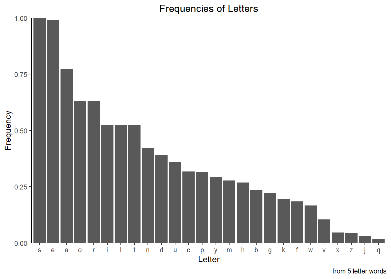
#plotting the frequency of the letters in our word_set
ggplot(char_frequencies,
       aes(x = fct_rev(fct_reorder(letters,  normalized)), y = normalized )) +
  geom_col() +
  theme_classic() +
  theme(legend.position = "none") +
  labs(title = "Frequencies of Letters", caption = "from 5 letter words") +
  theme(plot.title = element_text(hjust = 0.5)) +
  xlab("Letter") +
  ylab("Frequency") +
    scale_y_continuous(expand = c(0, 0))
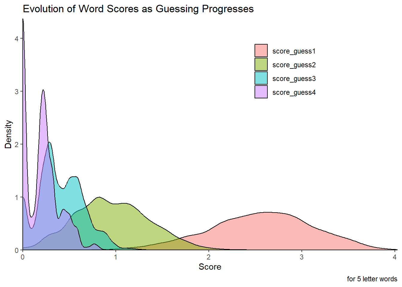
## This looks at the distribution of scores as guessing occurs.  Initially, you have a

word_scores_reshaped$score_type <- as.factor(word_scores_reshaped$score_type)

ggplot(word_scores_reshaped, aes(score, fill = score_type)) +
  geom_density(alpha = 0.5) +
  theme_classic() +
  labs(title = "Evolution of Word Scores as Guessing Progresses",
       caption = "for 5 letter words") +
  xlab("Score") +
  ylab("Density") +
  labs(fill = "") +
  theme(legend.position = c(0.7, 0.8)) +
  scale_x_continuous( expand = c(0, 0)) +
scale_y_continuous( expand = c(0, 0)) 
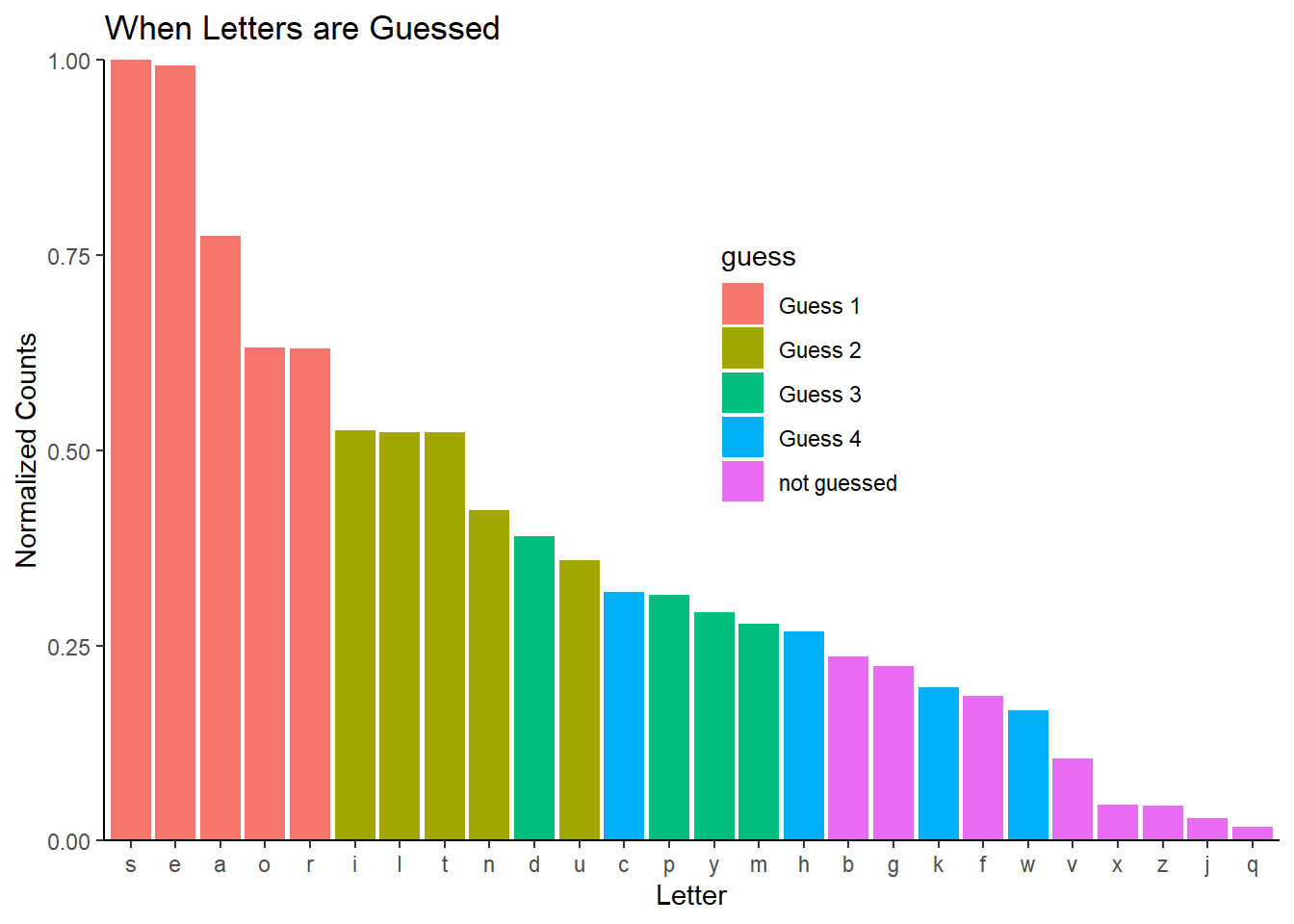
## Now we are visualizing what letters are picked in each guess
guess <- rep("not guessed", times = 26)
char_frequencies <- cbind(char_frequencies, guess)

# this is done in reverse order because some letters are guessed in more than
# one word and I'd like them marked at the earliest guess.
letter_vec <-  unlist(strsplit(word_4, split = ""))
print(letter_vec)
[1] "w" "h" "a" "c" "k"for (i in 1:length(letter_vec)) {
position <- letter_vec[i] == char_frequencies$letters
char_frequencies$guess[position] <- "Guess 4"
}
letter_vec <- unlist(strsplit(word_3, split = ""))
print(letter_vec)[1] "d" "u" "m" "p" "y"for (i in 1:length(letter_vec)) {
position <- letter_vec[i] == char_frequencies$letters
char_frequencies$guess[position] <- "Guess 3"
}
letter_vec <- unlist(strsplit(word_2, split = ""))
print(letter_vec)[1] "u" "n" "t" "i" "l"for (i in 1:length(letter_vec)) {
position <- letter_vec[i] == char_frequencies$letters
char_frequencies$guess[position] <- "Guess 2"
}
letter_vec <- unlist(strsplit(word_1, split = ""))
print(letter_vec)[1] "a" "r" "o" "s" "e"for (i in 1:length(letter_vec)) {
position <- letter_vec[i] == char_frequencies$letters
char_frequencies$guess[position] <- "Guess 1"
}
ggplot(char_frequencies, aes(
x = fct_rev(fct_reorder(letters, normalized)),
y = normalized,
fill = guess)) +
geom_col() +
ggtitle("When Letters are Guessed") +
ylab("Normalized Counts") +
xlab("Letter") +
theme_classic() +
theme(legend.position = c(0.6, 0.6)) +
scale_y_continuous(expand = c(0, 0))
So that’s the current state of this project. This was a really useful project for me and it really strengthened by R and Tidyverse skills.
Citation
@online{sinks2023,
  author = {Sinks, Louise E.},
  title = {Self-Guided {Learning} Through a {Wordle} {Guess}
    {Generator:} {Part} 2},
  date = {2023-04-01},
  url = {https://lsinks.github.io/posts/2023-04-01-self-guided-learning-wordle-guesser-part-2/current_wordle.html},
  langid = {en}
}