TidyTuesday Week 12: Programming Languages Revisited

TidyTuesday

R-code

code-along

data visualization

skimr

TidyTuesday: Polishing

Author

Louise E. Sinks

Published

March 24, 2023

Modified

November 3, 2023

This week, I participated in my first #TidyTuesday challenge. My goal was to get something out on the day of the challenge rather than perfection. I did notice that the skimr output wasn’t formatted nicely on the webpage. Today, I’m going to delve into the skimr and Quarto documentation and make a nicer version of the output. Secondly, I’m going to fix up my final figure, which is the one I shared on social media:

My first try at a #TidyTuesday challenge. We were given a dataset about what characters are used to comment computer code. This viz shows the most “highly ranked” language for each type of commenting token. The size of the word reflects the # of users of that language. #RStats pic.twitter.com/oGhqaYHD5U

— Louise Sinks (@LouiseSinks) March 21, 2023

Skimr to understand your data

Skimr is a package that provides statistical summaries of the variables in your dataframe. It also provides information about the missingness of each variable.

library(tidytuesdayR)
library(tidyverse)
library(skimr)
library(ggthemes)
library(gt)
library(ggrepel)
library(visdat) # visualizing missing data in dataframe

# Get the Data

# Read in with tidytuesdayR package 
# This loads the readme and all the datasets for the week of interest

# Either ISO-8601 date or year/week works!

#tuesdata <- tidytuesdayR::tt_load('2023-03-21')
tuesdata <- tidytuesdayR::tt_load(2023, week = 12)

languages <- tuesdata$languages

Customizing the skim Output

My main objection is that the numerical summary is too wide and has a scroll bar. I especially want the histogram to be viewable on the first screen. I also don’t particularly care about all the quartile information; min and max are enough. If I want to delve more into the stats of a variable, I will do it another way, not with skimr.

First, quarto lets you expand the output of the code chunk to fill the page via the option “#| column: page”, so I’ll do that. Next, I’ll create a custom skim function that drops the p25, p50, and p75 output from the summary of the numerical variables.

my_skim <- skim_with(numeric = sfl(p25 = NULL, p50 = NULL, p75 = NULL)) 

my_skim(languages)

Data summary
Name	languages
Number of rows	4303
Number of columns	49
_______________________
Column type frequency:
character	21
logical	4
numeric	24
________________________
Group variables	None

Variable type: character

skim_variable	n_missing	complete_rate	min	max	n_unique
pldb_id	0	1.00	1	52	4303
title	0	1.00	1	56	4267
description	3480	0.19	4	2273	811
type	0	1.00	2	27	40
creators	3203	0.26	2	253	985
website	2928	0.32	13	131	1368
domain_name	3588	0.17	6	32	700
reference	2314	0.46	15	251	1955
github_repo	3402	0.21	25	73	897
github_repo_description	3438	0.20	4	419	853
github_language	3829	0.11	1	30	474
github_language_tm_scope	3837	0.11	4	34	361
github_language_type	3837	0.11	4	11	4
github_language_ace_mode	3838	0.11	1	16	96
github_language_file_extensions	3833	0.11	1	606	466
wikipedia	2731	0.37	32	104	1566
wikipedia_summary	2884	0.33	17	6741	1407
wikipedia_related	3145	0.27	1	1761	1059
line_comment_token	3831	0.11	1	7	23
origin_community	1190	0.72	3	305	2232
file_type	3213	0.25	2	6	4

Variable type: logical

skim_variable	n_missing	complete_rate	mean	count
features_has_comments	3683	0.14	1.00	TRU: 617, FAL: 3
features_has_semantic_indentation	3722	0.14	0.11	FAL: 516, TRU: 65
features_has_line_comments	3765	0.13	0.96	TRU: 517, FAL: 21
is_open_source	3792	0.12	0.89	TRU: 453, FAL: 58

Variable type: numeric

skim_variable	n_missing	complete_rate	mean	sd	p0	p100	hist
appeared	0	1.00	1991.11	111.44	-2000	2023	▁▁▁▁▇
domain_name_registered	3801	0.12	2011.33	7.02	1990	2023	▁▃▃▇▆
isbndb	3217	0.25	7.71	33.16	0	400	▇▁▁▁▁
book_count	0	1.00	2.08	17.34	0	401	▇▁▁▁▁
semantic_scholar	3545	0.18	3.79	8.32	0	52	▇▁▁▁▁
language_rank	0	1.00	2151.00	1242.31	0	4302	▇▇▇▇▇
github_repo_stars	3414	0.21	2127.40	7554.02	0	88526	▇▁▁▁▁
github_repo_forks	3417	0.21	261.29	1203.00	0	23732	▇▁▁▁▁
github_repo_updated	3418	0.21	2021.39	1.76	2012	2023	▁▁▁▁▇
github_repo_subscribers	3418	0.21	62.34	200.88	0	2910	▇▁▁▁▁
github_repo_created	3425	0.20	2015.84	3.48	2006	2022	▁▅▇▇▇
github_repo_issues	3518	0.18	123.03	546.26	0	9522	▇▁▁▁▁
github_repo_first_commit	3567	0.17	2014.74	4.99	1987	2022	▁▁▁▆▇
github_language_repos	3833	0.11	197134.67	1226900.57	0	16046489	▇▁▁▁▁
wikipedia_daily_page_views	2837	0.34	227.13	783.55	-1	13394	▇▁▁▁▁
wikipedia_backlinks_count	2877	0.33	318.55	1635.29	1	34348	▇▁▁▁▁
wikipedia_page_id	2893	0.33	9167847.21	13506832.90	928	63063548	▇▁▁▁▁
wikipedia_appeared	2958	0.31	1991.14	17.03	1830	2019	▁▁▁▃▇
wikipedia_created	3040	0.29	2005.75	3.77	2001	2020	▇▇▂▁▁
wikipedia_revision_count	3130	0.27	330.43	813.26	1	10104	▇▁▁▁▁
last_activity	0	1.00	2000.62	84.60	-900	2023	▁▁▁▁▇
number_of_users	0	1.00	13771.26	227712.95	0	7179119	▇▁▁▁▁
number_of_jobs	0	1.00	422.18	12572.99	0	771996	▇▁▁▁▁
central_package_repository_count	1482	0.66	0.00	0.00	0	0	▁▁▇▁▁

This output is much nicer. It is a bit wall of text though. I wouldn’t recommend using this in reports, but it is a useful tool when doing your initial dataset analysis. (As a side note, I have noticed skimr doesn’t work well on Kaggle. It performs as expected if you are in interactive mode, but it fails when you try to save the notebook or run non-interactively.)

Styling skim output with gt

If, for some reason, you did need to include output/ visualizations about missingness in a report, I’d probably recreate visualizations or tables by class of variable, especially if you have many variables, as I do here.

Here’s an example for numeric variables, of which there are 24 in the dataset. First, we will skim the data and then use the gt package to style the resulting dataframe as a table. I used a built-in style, but each table element can be individually customized.

languages_numeric <- languages %>%
  select_if(is.numeric)

lang_numeric_skim <- my_skim(languages_numeric)

lang_numeric_skim %>%
  select(-skim_type)   %>% 
  gt() %>%
  cols_label(n_missing = "# Missing", complete_rate = "Completeness", 
             numeric.mean = "Mean", numeric.sd = "Standard Deviation",
             numeric.p0 = "Min", numeric.p100 = "Max",
             numeric.hist = "Histogram") %>%
  opt_stylize(style = 6, color = "blue", add_row_striping = TRUE) %>%
  tab_header(title = "Summary of Numerical Variables in Languages")

skim_variable	# Missing	Completeness	Mean	Standard Deviation	Min	Max	Histogram
Summary of Numerical Variables in Languages
appeared	0	1.0000000	1.991105e+03	1.114434e+02	-2000	2023	▁▁▁▁▇
domain_name_registered	3801	0.1166628	2.011333e+03	7.021132e+00	1990	2023	▁▃▃▇▆
isbndb	3217	0.2523821	7.706262e+00	3.316421e+01	0	400	▇▁▁▁▁
book_count	0	1.0000000	2.079479e+00	1.734465e+01	0	401	▇▁▁▁▁
semantic_scholar	3545	0.1761562	3.794195e+00	8.316231e+00	0	52	▇▁▁▁▁
language_rank	0	1.0000000	2.151000e+03	1.242313e+03	0	4302	▇▇▇▇▇
github_repo_stars	3414	0.2066000	2.127403e+03	7.554016e+03	0	88526	▇▁▁▁▁
github_repo_forks	3417	0.2059029	2.612867e+02	1.203003e+03	0	23732	▇▁▁▁▁
github_repo_updated	3418	0.2056705	2.021390e+03	1.763285e+00	2012	2023	▁▁▁▁▇
github_repo_subscribers	3418	0.2056705	6.234237e+01	2.008820e+02	0	2910	▇▁▁▁▁
github_repo_created	3425	0.2040437	2.015843e+03	3.479589e+00	2006	2022	▁▅▇▇▇
github_repo_issues	3518	0.1824309	1.230344e+02	5.462553e+02	0	9522	▇▁▁▁▁
github_repo_first_commit	3567	0.1710435	2.014739e+03	4.985409e+00	1987	2022	▁▁▁▆▇
github_language_repos	3833	0.1092261	1.971347e+05	1.226901e+06	0	16046489	▇▁▁▁▁
wikipedia_daily_page_views	2837	0.3406925	2.271330e+02	7.835524e+02	-1	13394	▇▁▁▁▁
wikipedia_backlinks_count	2877	0.3313967	3.185484e+02	1.635289e+03	1	34348	▇▁▁▁▁
wikipedia_page_id	2893	0.3276784	9.167847e+06	1.350683e+07	928	63063548	▇▁▁▁▁
wikipedia_appeared	2958	0.3125726	1.991144e+03	1.702650e+01	1830	2019	▁▁▁▃▇
wikipedia_created	3040	0.2935162	2.005748e+03	3.768240e+00	2001	2020	▇▇▂▁▁
wikipedia_revision_count	3130	0.2726005	3.304314e+02	8.132556e+02	1	10104	▇▁▁▁▁
last_activity	0	1.0000000	2.000616e+03	8.459776e+01	-900	2023	▁▁▁▁▇
number_of_users	0	1.0000000	1.377126e+04	2.277129e+05	0	7179119	▇▁▁▁▁
number_of_jobs	0	1.0000000	4.221838e+02	1.257299e+04	0	771996	▇▁▁▁▁
central_package_repository_count	1482	0.6555891	0.000000e+00	0.000000e+00	0	0	▁▁▇▁▁

Visualizing Missingness with visdat

The visdat package makes ggplot- compatible missingness plots. The cluster = TRUE option groups variables that share missingness. Here we see that usually if some of the GitHub data is missing, then all of the GitHub data is missing. The percent missing is listed for each variable, and the overall missingness of the dataset is shown in the legend.

Note vis_miss doesn’t work on very large datasets. The documentation suggests keeping the number of records below 1,000. A more extensive package for exploratory visualizations called naniar could also be used.

languages_numeric %>%
vis_miss(cluster = TRUE) +
ggtitle("Missing Data in the Languages Dataset") +
  #theme_classic() +
  theme(axis.text.x = element_text(size = 8, angle = 90))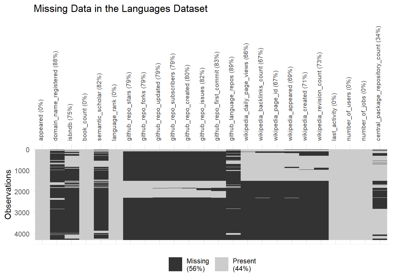

Improving “The Most Popular Language for Each Comment Token” Figure

joined <- read_csv("processed_lang.csv" , show_col_types = FALSE)

Now the original figure:

joined %>%
  ggplot(aes(line_comment_token, n, size = log(number_of_users), 
             color = log(number_of_users), label = title)) +
 # geom_point() +
  scale_y_log10() +
  geom_text_repel(show.legend = FALSE) +
   ggtitle("The Most Popular Language for Each Comment Token") +
  xlab("Token") +
  ylab("Number of languages using token") +
  theme_classic()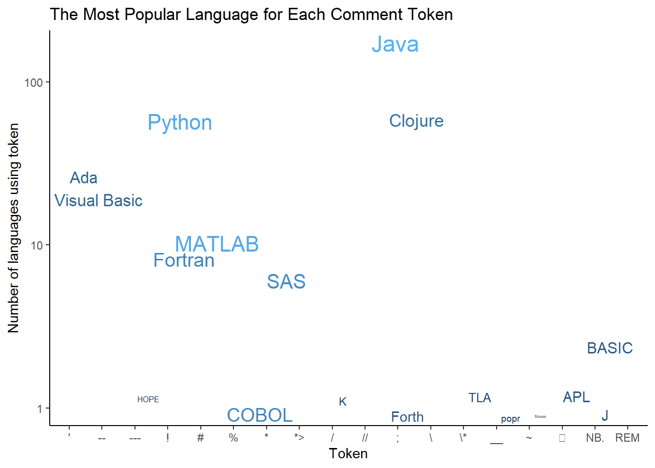

I thought I had noted this in the previous post, but one of the tokens, ⍝ , is rendered as an empty box in the ggplot figures. I thought fixing this would be easy. First, I thought I could just pass the Unicode value for that symbol. Then, when that didn’t work, I thought I could change the font to one supporting that symbol. Supposedly, changing the font should be easy, yet after 3 hours working on it, I still had blank squares. There is a nice tutorial on changing fonts in ggplot that did not work until I found someone with the same issue. The solution is to add a line of code that doesn’t make much sense to me : windowsFonts("Cambria Math" = windowsFont("Cambria Math"))

I saw a nice TidyTuesday figure on Twitter:

My submission for #TidyTuesday, Week 12 on programming languages. I explore jobs per users.

Code: https://t.co/bV9DUHZmro pic.twitter.com/2D5YLnE5yz

— Mitsuo Shiota (@mitsuoxv) March 21, 2023

with a caption referencing the original dataset. I’d like to add that. I generally want to increase the figure’s legibility and flip the color scale so that darker blue corresponds to more users. I also don’t think what popular means is entirely clear, so I’d like to explain more fully what I’m graphing.

windowsFonts("Cambria Math" = windowsFont("Cambria Math"))
joined %>%
  ggplot(aes(line_comment_token, n, size = log(number_of_users), 
             color = log(number_of_users), label = title)) +
  scale_y_log10() +
  geom_text_repel(show.legend = FALSE) +
    scale_colour_gradient(high = "#08306b", low = "#6baed6") + 
   labs(title = "The Most Popular Language for Each Comment Token",
       subtitle = "Based on # Users and Rank",
       caption = "data from https://pldb.com/") +
  xlab("Token") +
  ylab("Number of languages using token") +
  theme_classic(base_size = 16) +
  theme(text = element_text( family = "Cambria Math")) +
  theme(axis.text.x = element_text(face = "bold"))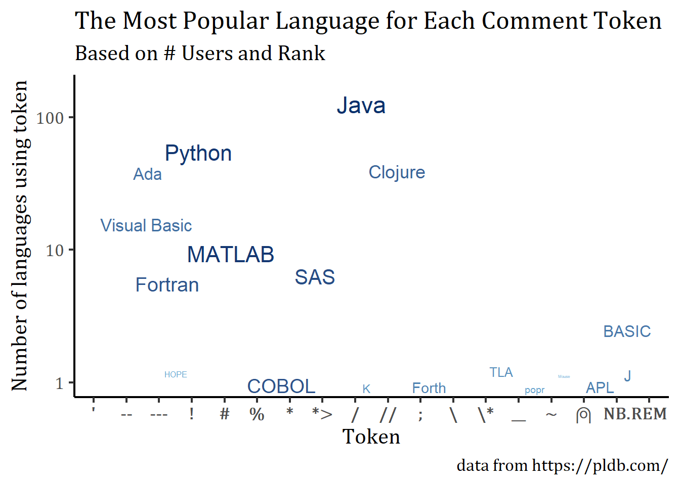

Citation

BibTeX citation:

@online{sinks2023,
  author = {Sinks, Louise E.},
  title = {TidyTuesday {Week} 12: {Programming} {Languages} {Revisited}},
  date = {2023-03-24},
  url = {https://lsinks.github.io/posts/2023-03-24-tidytuesday-figure-polishing/},
  langid = {en}
}

For attribution, please cite this work as:

Sinks, Louise E. 2023. “TidyTuesday Week 12: Programming Languages Revisited.” March 24, 2023. https://lsinks.github.io/posts/2023-03-24-tidytuesday-figure-polishing/.